Modelo de regresión polinomial

Metodología

Los pasos a seguir para alcanzar el objetivo son los siguientes:

1. Importación de la base de datos.

2. Análisis de las variables para identificar el tipo de dato.

3. Verificación de valores NaN o Nulos.

4. Distribución de las variables.

5. Cálculo de la matriz de correlación.

6. Procesamiento de datos.

7. Resultados y discusión.

Configuración

Importación de librerías

Importamos todas las librerías necesarias para trabajar

import numpy as np
import pandas as pd
import seaborn as sns
import matplotlib.pyplot as plt

from sklearn import preprocessing
from sklearn.linear_model import LinearRegression
from sklearn.preprocessing import PolynomialFeatures
from sklearn.model_selection import train_test_split
from sklearn.metrics import mean_squared_error, mean_absolute_error, r2_score, explained_variance_score

# 1. Importación de la base de datos
dataset = pd.read_csv('datasets/ground_source_heat_pump.csv')
dataset.head()

	HEM	STC	VWD	WD	UT	WFR	WTD	HTR
0	Release	1.41	100.0	180	3.0	1.15	4.04	53.9
1	Release	1.41	125.0	180	3.0	1.15	4.86	52.0
2	Extraction	1.41	100.0	180	3.0	1.15	3.18	42.4
3	Extraction	1.41	125.0	180	3.0	1.15	3.82	40.7
4	Release	1.46	85.0	130	2.8	1.19	4.19	66.6

# 2. Análisis de las variables para identificar el tipo de dato
dataset.info()

<class 'pandas.core.frame.DataFrame'>
RangeIndex: 112 entries, 0 to 111
Data columns (total 8 columns):
 #   Column  Non-Null Count  Dtype  
---  ------  --------------  -----  
 0   HEM     112 non-null    object 
 1   STC     112 non-null    float64
 2   VWD     112 non-null    float64
 3   WD      112 non-null    int64  
 4   UT      112 non-null    float64
 5   WFR     112 non-null    float64
 6   WTD     112 non-null    float64
 7   HTR     112 non-null    float64
dtypes: float64(6), int64(1), object(1)
memory usage: 7.1+ KB

# 3. Verificación de valores NaN o nulos
dataset.isnull().sum()

HEM    0
STC    0
VWD    0
WD     0
UT     0
WFR    0
WTD    0
HTR    0
dtype: int64

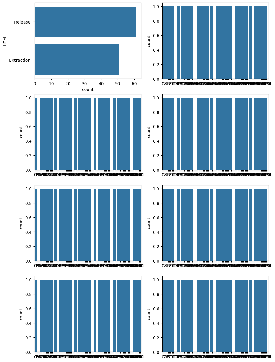
# 4. Distribución de las variables
cols = dataset.columns
fig, axes = plt.subplots(4,2, figsize = (10,15))
k = 0

for i in range(4):
    for j in range(2):
        sns.countplot(dataset[cols[k]], ax = axes[i][j])
        k = k + 1

# 5. Cálculo de la matriz de correlación
fig = plt.figure(figsize = (10,10))
sns.heatmap(dataset[dataset.keys().drop('HEM')].corr(), annot = True)

<Axes: >

scaler = preprocessing.MinMaxScaler(feature_range = (0.1, 0.9))
X = PolynomialFeatures(degree=2, include_bias=False).fit_transform(scaler.fit_transform(dataset[dataset.keys().drop(['HEM','HTR'])]))
y = np.asarray(dataset['HTR'])

X_train, X_test, y_train, y_test = train_test_split(X, y, test_size = 0.20)

#%% Specify the model
model = LinearRegression()

#%% Fit model on the dataset
model.fit(X_train, # input data
            y_train, # target data
            )

LinearRegression()

In a Jupyter environment, please rerun this cell to show the HTML representation or trust the notebook.
On GitHub, the HTML representation is unable to render, please try loading this page with nbviewer.org.

# Predict on training data
pred_tr = model.predict(X_train)

# Predict on a test data
pred_te = model.predict(X_test)

def regression_results(y_true, y_pred):
    # Regression metrics
    ev = explained_variance_score(y_true, y_pred)
    mae = mean_absolute_error(y_true, y_pred) 
    mse = mean_squared_error(y_true, y_pred) 
    r2 = r2_score(y_true, y_pred)

    print('explained_variance: ', round(ev,4))    
    print('MAE: ', round(mae,4))
    print('MSE: ', round(mse,4))
    print('R²: ', round(r2,4))

#%% Model Performance Summary    
print("")
print('---------- Evaluation on Training Data ----------')
regression_results(y_train, pred_tr)
print("")

print('---------- Evaluation on Test Data ----------')
regression_results(y_test, pred_te)
print("")

#%% Results per output
mse_train = mean_squared_error(y_train, pred_tr)

r2_train = r2_score(y_train, pred_tr)

mse_test = mean_squared_error(y_test, pred_te)

r2_test = r2_score(y_test, pred_te)

col_names = ('MSE (train)', 'R2 (train)', 'MSE (test)', 'R2 (test)')

df = np.array([mse_train, r2_train, mse_test, r2_test])

print("")
print('---------- Evaluation per output ----------')
results = pd.DataFrame(data = df.reshape(1,-1), columns = col_names)
print(results)

---------- Evaluation on Training Data ----------
explained_variance:  0.8902
MAE:  2.2453
MSE:  10.1288
R²:  0.8902

---------- Evaluation on Test Data ----------
explained_variance:  0.4955
MAE:  4.5854
MSE:  42.9591
R²:  0.4879


---------- Evaluation per output ----------
   MSE (train)  R2 (train)  MSE (test)  R2 (test)
0    10.128808     0.89023    42.95908   0.487884