Sistemas de ED lineales de primer orden
Un sistema de ED de primer orden de la forma normal
\[\begin{split}
\begin{aligned}
\frac{\mathrm{d}x_{1}}{\mathrm{d}t} &= g_{1}\left( t,x_{1},x_{2},\dots,x_{n} \right), \\
\frac{\mathrm{d}x_{2}}{\mathrm{d}t} &= g_{2}\left( t,x_{1},x_{2},\dots,x_{n} \right), \\
\vdots \quad &= \qquad \vdots \\
\frac{\mathrm{d}x_{n}}{\mathrm{d}t} &= g_{n}\left( t,x_{1},x_{2},\dots,x_{n} \right),
\end{aligned}
\end{split}\]
se llama sistema de primer orden .
Cuando las funciones \(g_{1},g_{2},\dots,g_{n}\) son lineales en las variables dependientes \(x_{1},x_{2},\dots,x_{n}\) se obtiene la forma normal de un sistema de ecuaciones lineales de primer orden de la forma
(45) \[\begin{split}
\begin{aligned}
\frac{\mathrm{d}x_{1}}{\mathrm{d}t} &= a_{11}x_{1}(t) + a_{12}x_{2}(t) + \cdots + a_{1n}x_{n}(t) + f_{1}(t), \\
\frac{\mathrm{d}x_{2}}{\mathrm{d}t} &= a_{21}x_{1}(t) + a_{22}x_{2}(t) + \cdots + a_{2n}x_{n}(t) + f_{2}(t), \\
\vdots \quad &= \qquad \qquad \qquad \qquad \qquad \vdots \\
\frac{\mathrm{d}x_{n}}{\mathrm{d}t} &= a_{n1}x_{1}(t) + a_{n2}x_{2}(t) + \cdots + a_{nn}x_{n}(t) + f_{n}(t). \\
\end{aligned}
\end{split}\]
Cuando \(f_{i}(t) = 0\) , para \(i=1,2,\dots,n\) , se dice que el sistema lineal (45) es homogéneo ; en caso contrario es no homogéneo .
Si definimos las siguientes matrices
\[\begin{split}
{\bf X} := \begin{bmatrix} x_{1}(t) \\ x_{2}(t) \\ \vdots \\ x_{n}(t) \end{bmatrix}, \quad {\bf A} := \begin{bmatrix} a_{11} & a_{12} & \cdots & a_{1n} \\ a_{21} & a_{22} & \cdots & a_{2n} \\ \vdots & \vdots & \ddots & \vdots \\ a_{n1} & a_{n2} & \cdots & a_{nn} \end{bmatrix}, \quad {\bf F} := \begin{bmatrix} f_{1}(t) \\ f_{2}(t) \\ \vdots \\ f_{n}(t) \end{bmatrix},
\end{split}\]
entonces el sistema dado en la Ec. (45) se puede escribir como
\[\begin{split}
\frac{\mathrm{d}}{\mathrm{d}t} \begin{bmatrix} x_{1} \\ x_{2} \\ \vdots \\ x_{n} \end{bmatrix} = \begin{bmatrix} a_{11} & a_{12} & \cdots & a_{1n} \\ a_{21} & a_{22} & \cdots & a_{2n} \\ \vdots & \vdots & \ddots & \vdots \\ a_{n1} & a_{n2} & \cdots & a_{nn} \end{bmatrix} \begin{bmatrix} x_{1} \\ x_{2} \\ \vdots \\ x_{n} \end{bmatrix} + \begin{bmatrix} f_{1}(t) \\ f_{2}(t) \\ \vdots \\ f_{n}(t) \end{bmatrix},
\end{split}\]
o bien
(46) \[
{\bf X'} = {\bf A}{\bf X} + {\bf F}.
\]
Ejemplo
Escriba los siguientes sistemas en notación matricial
\[\begin{split}
\begin{aligned}
\frac{\mathrm{d}x}{\mathrm{d}t} &= 3x + 4y, \\
\frac{\mathrm{d}y}{\mathrm{d}t} &= 5x - 7y.
\end{aligned}
\end{split}\]
\[\begin{split}
\begin{aligned}
\frac{\mathrm{d}x}{\mathrm{d}t} &= 6x + y + z + t, \\
\frac{\mathrm{d}y}{\mathrm{d}t} &= 8x + 7y - z + 10t, \\
\frac{\mathrm{d}z}{\mathrm{d}t} &= 2x + 9y - z + 6t.
\end{aligned}
\end{split}\]
Definition 10 (Vector solución)
Un vector solución en un intervalo \(I\) está definido como un vector columna
\[\begin{split}
{\bf X} = \begin{bmatrix} x_{1} \\ x_{2} \\ \vdots \\ x_{n} \end{bmatrix},
\end{split}\]
donde los elementos son funciones derivables que satisfacen el sistema (46) en el intervalo.
Para el caso de \(n=2\) , las ecuaciones \(x_{1} = \phi_{1}(t)\) y \(x_{2} = \phi_{2}(t)\) representan una trayectoria en el plano fase (plano \(x_{1}x_{2}\) ).
La solución general de un sistema homogéneo
(47) \[
{\bf X'} = {\bf A}{\bf X},
\]
es
(48) \[\begin{split}
{\bf X} = \begin{bmatrix} k_{1} \\ k_{2} \\ \vdots \\ k_{n} \end{bmatrix}e^{\lambda t} = {\bf K}e^{\lambda t},
\end{split}\]
donde \({\bf K}\) y \(\lambda\) son constantes.
Dado que (48) es un vector solución del sistema lineal homogéneo (47) , entonces
\[
{\bf X'} = {\bf A}{\bf K}e^{\lambda t},
\]
\[
{\bf K}\lambda e^{\lambda t} = {\bf A}{\bf K}e^{\lambda t}.
\]
Dividiendo ambos lados por el término \(e^{\lambda t}\) y realizando manipulaciones algebráicas se tiene
\[\begin{split}
\begin{aligned}
{\bf A}{\bf K} &= \lambda {\bf K}, \\
{\bf A}{\bf K} - \lambda {\bf K} &= 0.
\end{aligned}
\end{split}\]
Dado que \({\bf A}\) es una matriz de \(n\times n\) , entonces
\[
{\bf K} = {\bf I}{\bf K}.
\]
Por consiguiente
(49) \[
\left( {\bf A} - \lambda {\bf I} \right){\bf K} = 0.
\]
La solución \({\bf X}\) del sistema (47) depende de un vector no trivial \({\bf K}\) que satisfaga (49) . Por lo tanto, se debe considerar la siguiente ecuación característica de \({\bf A}\)
(50) \[
\text{det}\left( {\bf A} - \lambda {\bf I} \right) = 0,
\]
donde la solución de (50) son los eigenvalores de \({\bf A}\) .
Atención
Una solución \({\bf K} \neq 0\) se llama eigenvector de \({\bf A}\) y corresponde a un eigenvalor \(\lambda\) .
Entonces la solución del sistema homogéno (47) está dada por la siguiente expresión
\[
{\bf X} = {\bf K}e^{\lambda t}.
\]
Theorem 9 (Solución general de sistemas homogéneos)
Sean \(\lambda_{1},\lambda_{2},\dots,\lambda_{n}~\) \(n\) eigenvalores reales y diferentes de la matriz de coeficientes \({\bf A}\) y \({\bf K_{1}},{\bf K_{2}},\dots,{\bf K_{n}}\) sus eigenvalores correspondientes, entonces la solución general en el intervalo \((-\infty,\infty)\) está dada por
\[
{\bf X} = c_{1}{\bf K_{1}}e^{\lambda_{1}t} + c_{2}{\bf K_{2}}e^{\lambda_{2}t} + \cdots + c_{n}{\bf K_{n}}e^{\lambda_{n}t}.
\]
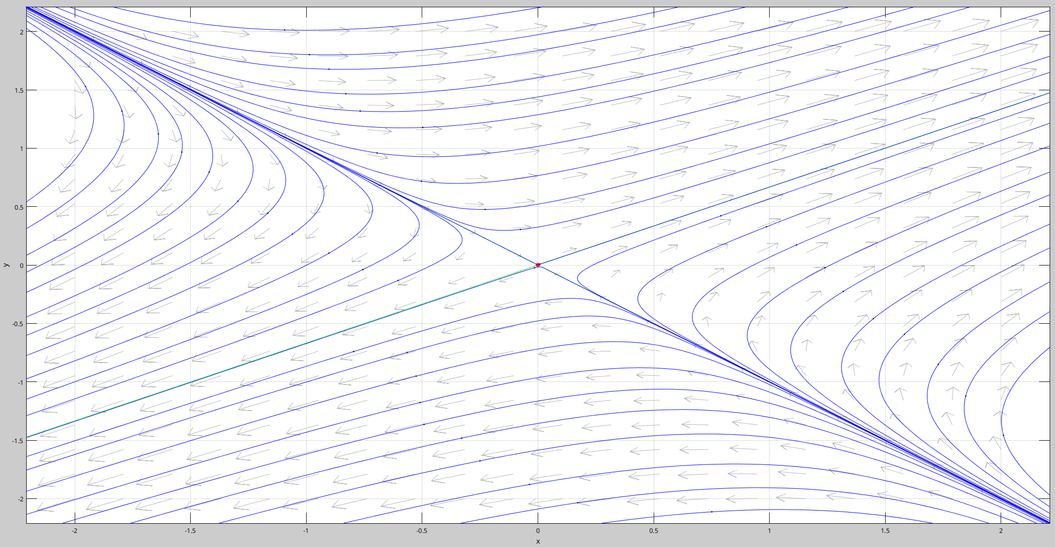
Diagramas de fase
Al conjunto de trayectorias en el plano fase como se muestra en la Figura 1 diagrama fase .
Figura 1 Diagrama fase del sistema péndulo simple.
Aquí se puede visualizar cada eigenvector como un vector bidimensional a lo largo de una de estas curvas.
Importante
El origen se le llama repulsor cuando \(\lambda_{1}>0,\lambda_{2}>0\) y atractor cuando \(\lambda_{1}<0,\lambda_{2}<0\) .
Ejemplo
Determine los eigenvalores y eigenvectores de los siguientes sistemas:
\[\begin{split}
\begin{aligned}
\frac{\mathrm{d}x}{\mathrm{d}t} &= 2x + 3y, \\
\frac{\mathrm{d}y}{\mathrm{d}t} &= 2x + y. \\
\end{aligned}
\end{split}\]
\[\begin{split}
\begin{aligned}
\frac{\mathrm{d}x}{\mathrm{d}t} &= -4x + y + z, \\
\frac{\mathrm{d}y}{\mathrm{d}t} &= x + 5y - z, \\
\frac{\mathrm{d}z}{\mathrm{d}t} &= y - 3z. \\
\end{aligned}
\end{split}\]
\[\begin{split}
{\bf X'} = \begin{bmatrix} 1 & -2 & 2 \\ -2 & 1 & -2 \\ 2 & -2 & 1 \end{bmatrix}{\bf X}.
\end{split}\]
\[\begin{split}
{\bf X'} = \begin{bmatrix} 2 & 1 & 6 \\ 0 & 2 & 5 \\ 0 & 0 & 2 \end{bmatrix}{\bf X}.
\end{split}\]
\[\begin{split}
\begin{aligned}
\frac{\mathrm{d}x}{\mathrm{d}t} &= 6x - y, \\
\frac{\mathrm{d}y}{\mathrm{d}t} &= 5x + 4y. \\
\end{aligned}
\end{split}\]
Theorem 10 (Soluciones correspondientes a un eigenvalor complejo)
Sea \({\bf X}\) una matriz de coeficientes con entradas reales de un sistema homogéneo y \({\bf K_{1}}\) el eigenvector correspondiente al eigenvalor complejo \(\lambda_{1} = \alpha + \beta i\) , con \(\alpha,\beta \in \mathbb{R}\) entonces
\[
{\bf K_{1}}e^{\lambda_{1}t}, \quad {\bf \overline{K}_{1}}e^{\overline{\lambda}_{1}t},
\]
son soluciones del sistema dado en la Ec. (47) .
Demuestre el Theorem 10 utilizando el siguiente PVI
\[\begin{split}
{\bf X'} = \begin{bmatrix} 2 & 8 \\ -1 & -2 \end{bmatrix}{\bf X}, \quad {\bf X}(0) = \begin{bmatrix} 2 \\ -1 \end{bmatrix}.
\end{split}\]